One of my recent favorite purchases was a Garmin Fenix 5 watch. I bought it primarily to track a European cycling trip from Regensburg, Germany to Vienna, Austria. But I've also enjoyed keeping track of the steps I take each day. In particular, I wondered what inferences I could make about my life using the step data from the past few months.

My wife and I recently got a puppy, Darcy. She's an energetic five-month-old, and to say our daily routines have changed as a result would be an understatement. My intuition was that I walked much more each day since Darcy arrived, and I wondered if the data, plus some Bayesian inference, would support my hypothesis. I was inspired by an example from Bayesian Methods for Hackers, by Cam Davidson-Pilon, where he examined text message patterns over a period of time.

The question:

Concretely, I want to determine if my step behavior changed over time. Was there a specific day or range of days where my activity increased or decreased? How much did my steps change? If I observed a change, what could I attribute it to?

I'll use the excellent pymc3 library to construct a model to answer my question. The model consists of prior assumptions about the distribution of my steps as well as an inference engine to fit my data and estimate a posterior distribution. The posterior distribution will be used to estimate the likelihood that my behavior changed.

The data:

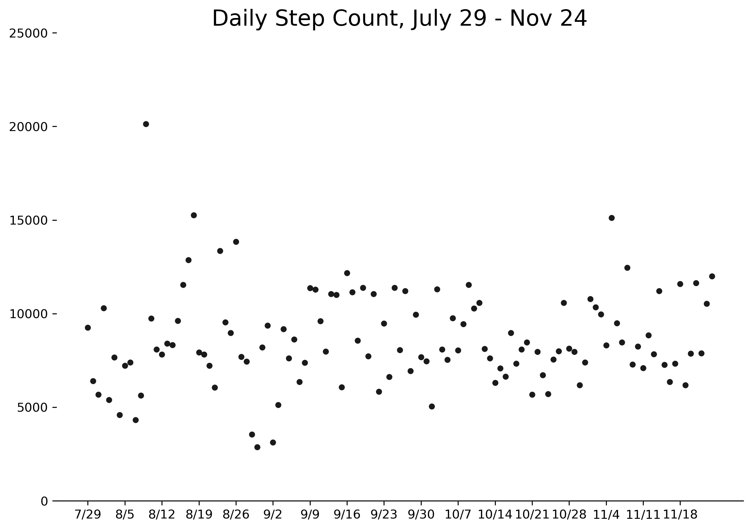
The first step was to gather the data from my Garmin watch. Unsurprisingly, this was not a very exciting process, but I eventually collected several months of step data, starting from the end of July. As data goes, it's quite simple: a column for the actual steps logged each day, and a column for that day's goal. (Garmin uses an algorithm to set an adjustable daily step goal. I was curious about the logic behind the algorithm, but I'll save it for another post.) The data looks something like this:

             actual    goal
2018-07-29     9250    7140
2018-07-30     6392    7360
2018-07-31     5668    7270
2018-08-01    10286    6950
...             ...     ...
2018-11-22     7888    8520
2018-11-23    10532    8460
2018-11-24    11999    8670

You can find the complete data - all 119 days of it - here. Please feel free to replicate or expand this analysis as you wish, but I'd love to hear about what you do. Find me on Twitter or email me your results!

The priors:

I start by assuming my steps are normally distributed. From the sample data, I calculated $mu=8637$ and $sd=2559$. Technically speaking a normal distribution allows for the possibility of a negative daily step count at the extreme left tail, but the probability of this is roughly 0.04%. I'm willing to accept this for the ease of using the normal distribution (as opposed to a strictly-positive distribution like the lognormal) for modeling.

I suspect that my step activity increased after the puppy arrived, so I'll set up two normal distributions, $N_1$ and $N_2$, to represent models for my steps before and after that point. If my hypothesis is correct, then the mean of $N_2$ will be greater than the mean of $N_1$. A third variable, tau, will identify the point at which my steps shift from being modeled by $N_1$ to being modeled by $N_2$.

Each normal distribution is parameterized by a mean and standard deviation. I don't want to embed strong priors other than to force the mean and standard deviation to be positive numbers. Therefore, I'll model them using the exponential distribution. The exponential distribution takes a single parameter, alpha, which I'll set equal to the inverse of my sample mean and standard deviation, respectively. Similarly, I won't embed much prior knowledge about tau by assuming it is uniformly distributed across the entire time period.

The model:

Constructing this model with pymc3 is simple. I establish prior distributions for the parameters of the two normal distributions and let pymc3 run inference on the model. The output is a large batch of samples from the posterior distribution, which I can use to answer my questions about step behavior.

with pm.Model() as model:

    # parameterize the priors with sample mean and standard deviation
    alpha = 1 / data.actual.mean()
    beta = 1 / data.actual.std()

    # normal distribution priors - mu and std for before and after
    mu = pm.Exponential('mu', lam=alpha, shape=[2,])
    sd = pm.Exponential('sd', lam=beta, shape=[2,])

    t = np.arange(data.shape[0])
    tau = pm.DiscreteUniform('tau', lower=0, upper=t.max())
    _mu = pm.math.switch(tau > t, mu[0], mu[1])
    _sd = pm.math.switch(tau > t, sd[0], sd[1])

    observation = pm.Normal('observation', mu=_mu, sd=_sd, observed=data.actual)

    start = pm.find_MAP()
    trace = pm.sample(draws=5000, tune=5000, start=start)

The results

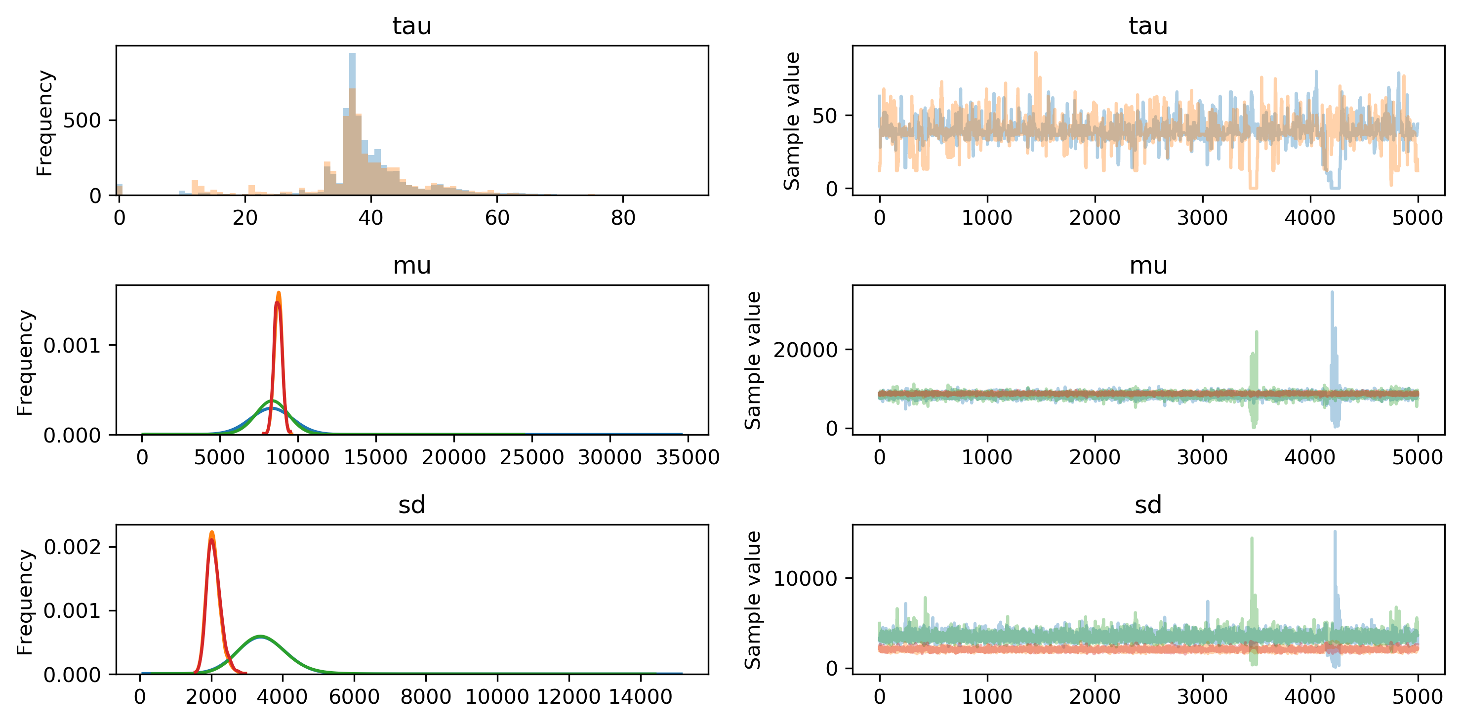
We can use the built-in visualization tools provided by pymc3 to examine the posterior distribution parameters. For example, the most likely value for tau is slightly less than 40 days, but appears to range anywhere from 30 to 50 days from the beginning of the time period. This suggests that the model did indeed identify a point at which my step data switched distributions.

More interesting, I think, are the parameters of the two normal distributions. The green lines represent mean and standard deviation of $N_1$, while red lines represent $N_2$. I noticed the $N_2$ mean appears to be slightly higher than $N_1$, but it doesn't look to be a significant difference. In fact, the average sampled means from $N_1$ and $N_2$ are 8335 and 8735 - a difference of just 400 steps per day.

However, the standard deviations of the normal distributions show much more divergence from each other. Prior to the switchpoint, the average standard deviation is 3452. After the switchpoint, it reduces to 2074.

What can we conclude from this? Originally I suspected that my step count increased after the puppy arrived. There appears to be some slight truth to this, given that the model predicted an average 400 steps extra per day, but that's not very convincing. In fact, using the maximum a posteriori values for $N_1$ and $N_2$ we can estimate how likely it would be for my step count to be higher on any given day after the puppy arrived. We sample repeatedly from each distribution and count the days where step count is higher from $N_2$.

# sample from both normal distribution 100,000 times
trials = 100000
samples = np.random.normal(loc=start['mu'], scale=start['sd'], size=(trials, 2))
results = sum(samples[:,1] > samples[:,0]) / trials

print(results)
0.49983

Based on this, it appears I was no likelier to walk farther after the puppy arrived. There was just a 50% chance that my step count would be higher with the puppy than it was before the puppy. This in and of itself is quite interesting: if I expect my average steps to be higher by 400 after the puppy, why isn't the likelihood greater than 50%?

It turns out that the higher standard deviation of $N_1$ means that I was more likely to see extremes on both ends of the spectrum: days with very few steps, and days with long hikes, like the 20,000 steps I recorded during a walking tour of Munich. Those high extremes compensated for the slightly lower average, making the probability nearly a coin flip overall. Of course this makes sense based on the distributions of $N_1$ and $N_2$, but counteracted my intuition.

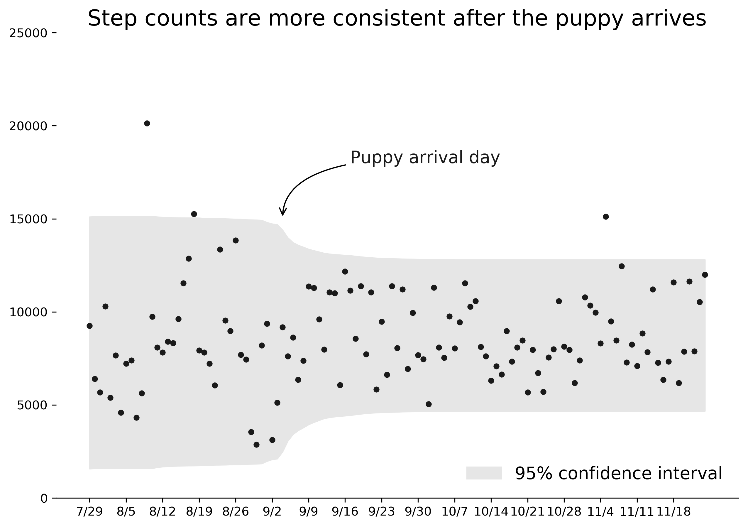
However, perhaps more importantly, the model suggested that the standard deviation of daily step count decreased, meaning the range of steps on a daily basis was much more consistent. Intuitively this feels like a better description of post-puppy life. Instead of significantly higher activity per day, my activity was more consistent: three or four regular daily walks and exercise to try to establish routine for Darcy.

I was impressed by the ability of the model to pinpoint the timing of this shift. The chart below shows the average 95% range of steps predicted per day by the model. There is a clear shift to a narrower range of results starting on the day we got our puppy and taking about a week to settle into a final band.

Therefore, though I wasn't able to prove that I walked more each day, I can say with confidence that the model accurately identified the timing and effect of Darcy on my activity level. Here's to many more years of walks with our puppy!